Dec 21, 2022

Trees and Tribulations

c# algorithms

A while ago we looked at two string-searching algorithms: a naive search and a version that is optimized for SIMD instructions. These algorithms are sufficient for searching short texts or looking for a single substring, but if you need to perform multiple searches over a longer text, such as a book, you may experience delays in the search results. To address this issue, there are faster string-searching algorithms that build indexing structures, like a suffix tree, during a preprocessing phase to speed up subsequent substring searches.

In this post, we will learn about suffix trees, build one using Ukkonen’s algorithm, and use it to search for strings. Suffix trees can be used for more than just string search, such as finding the longest repeated substring, the longest palindrome in a string, and implementing fuzzy string search (which we may cover in the future). Lately string processing algorithms have advanced significantly, particularly with the study of DNA sequences.

Before diving into the business of suffix trees, let’s first discuss a data structure called a trie, which will help us understand how suffix trees work.

Trie

A trie is a data structure that is often used to represent multiple strings in a single tree. Tries, also known as prefix trees, were previously used for implementing text suggestion before fancy AI took over. Let’s build a simple trie to see how it works using the following list of words as an example:

suede
muse
sum41
mud

We start by creating an empty root and adding the first word:

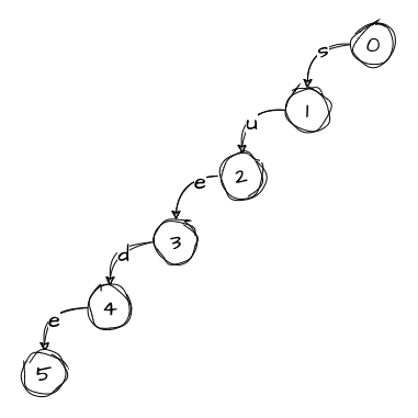
In the trie, a node holds a collection of edges, each representing a character. Since we only have one word in the trie so far, every node has only one edge. But this will change once we start adding more words.

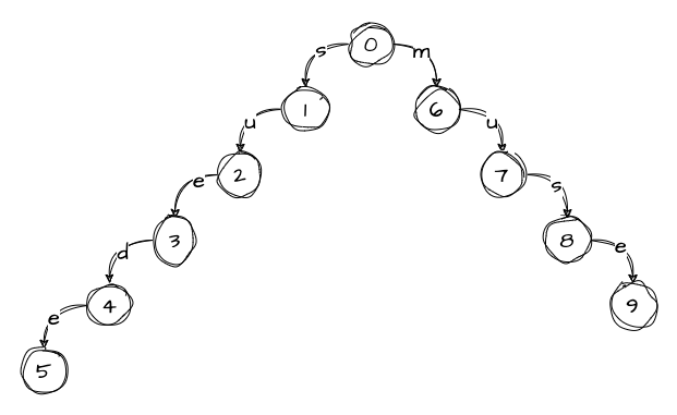
Next, we will add the second word:

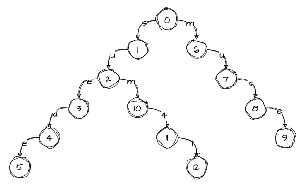
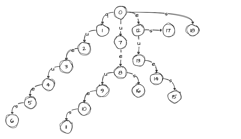
When we add the third word, we notice that we already have an edge labeled s that matches the first character of the word and points to node 1. We navigate to node 1 and continue down the tree, noting that we only need to add um41 to the tree. We also notice that we have another matching edge, u, that leads to node 2. We continue down the tree, keeping in mind that we only have m41 left to add:

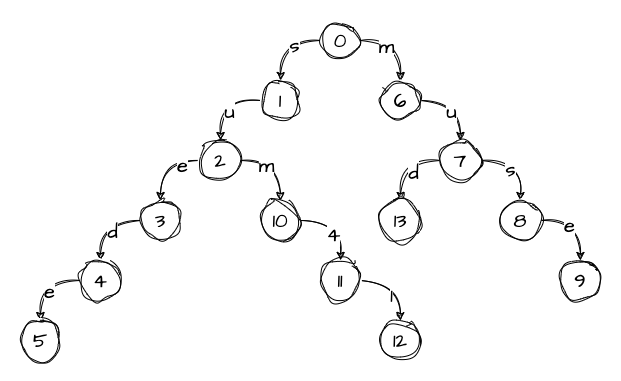
The same thing happens when we add the fourth word. We have an edge that matches the first character, so we proceed to node 6 with the rest of the word ud. Then we have another matching edge labeled u that leads us to node 7, leaving us with only d to add to the tree. Since there are no matching edges at this level, we add character d to the tree:

The trie is now ready to use. To query the trie, we start at the root and traverse the tree. For example, let’s say we want to find the string sum:

1. At the root level, we check if any edge holds the character s. We follow the edge labeled s and end up at node 1.
2. We repeat the previous step for the next character u, and end up at node 2.
3. Finally, we follow the edge labeled m and arrive at node 10, which concludes our traversal as we have reached the end of the query string.

By traversing the tree this way, we can determine that the trie contains the word sum. If we had not found a matching edge for a character in the query string, we would know that the word is not in the trie.

Hang on a second, I hear you say, earlier in the post, we were talking about string search. How do a list of words, a trie, and prefix search help us with that? To answer that, we need to convert our trie, also known as a prefix tree, into a suffix tree.

Suffix Tree

Suppose we have a string queues and want to search for substrings like eu or es. To do this, we first need to extract all possible suffixes of the source string:

queues
ueues
eues
ues
es
s

Now we can see that any substring that exists in the string will be a prefix of one of the suffixes. We can use this observation to build a trie containing all the suffixes and then use the same tree traversal algorithm we used before to search for a substring:

As we can see, there are many “internal” nodes between the root and the leaves that have a single child. We can compress the tree by combining the values of these edges into a single edge and removing the nodes in-between:

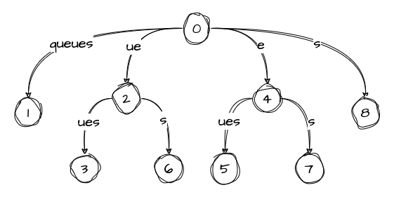
This compressed tree is also called a radix tree. We can also save some space by replacing substrings that lie on the edges with intervals that point to the start and end of the substrings:

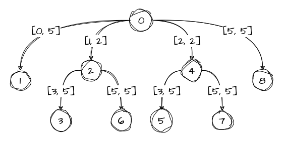
Now we have a performance issue to consider. While we can query a suffix tree in linear time O(m), where m is the length of the string we want to search for, by simply walking down the tree and following the correct edge, constructing the tree is somewhat slow. This is because we need to build the tree and then compress it, which increases the time complexity to O(n^2), where n is the number of characters in the source text.

To address this issue, we can use Ukkonen’s algorithm to construct a suffix tree in linear time.

Ukkonen’s Algorithm

Some say that Ukkonen’s algorithm is a bit hard to grasp. In my opinion, it may not be immediately intuitive and may require a couple of read-throughs to fully grasp, but it — appologies for the double negative — is not incomprehensible. On Stack Overflow, there is an excellent thread containing various explanations and implementations of the algorithm that may help with understanding how it works. It’s by far and away the best resource I found on the topic, I highly recommend reading it.

We will analyze the algorithm using the word velvetveil that contains multiple repeating characters as an example. (Something like velvetrevolver would, of course, be more appropriate to be on par with previous examples, but we will try to keep the example short and simple.) As you may have noticed, it’s actually two words, but since the space is just another character, we remove it for simplicity. We start constructing the tree from the first character v, progressing to the end until we reach the last l.

Before we start with the first character, we need to introduce two helper variables: the remainder and the active point.

The remainder keeps track of how many suffixes we need to add during each step. As we go through the string character by character, we consider each character to be a suffix. However, if we encounter a character that is already present in the tree, we increment the remainder, meaning that we will need to take it into account when processing the next character.

The active point is a triple that consists of three values: active_node, active_edge, and active_length. It also comes with three additional rules that we must follow:

1. If we insert a new node from the root, the following actions should take place:
   • active_node remains the root.
   • active_edge is set to the first character of the suffix we need to insert next.
   • active_length is decremented.
2. If we insert a new node and it’s not the first node created during the current step, we connect the previously inserted node and the new node through a suffix link.
3. After creating a new node from an active_node that is not the root node, we follow the suffix link going out of that node, if there is one, and reset the active_node to the node it points to. If there is no suffix link, we set the active_node to the root. active_edge and active_length remain unchanged.

These rules may not be immediately obvious, but later we will see how they help us construct the tree. We can think of the active point as a sliding window that moves through the string and shows us where in the tree we need to insert a new node. At each step, the suffix represented by the sliding window is added to the tree. The active point is the key element of the algorithm that helps us construct the tree in linear time.

Now let’s start constructing the suffix tree. We will have 10 steps, each step being responsible for a character. Let’s mark the current step as # and note that each edge holds an interval pointing to a substring within the source string. For example, an interval [0,2] would point to the word vel.

Step 0

Before we start working with the word, we need to create a root node, initialize the active point, and set the remainder to 0:

remainder: 0
active_node: 0
active_edge: ''
active_length: 0

Step 1: v

The first character v can be easily added to the tree: we create a new node and connect it to the root with an edge, marking the edge with the position of v in the string:

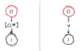
The tree on the left shows how we model it, and the tree on the right shows how we can visualize it. All variables have the same values.

Step 2: ve

The second character e creates a new node and a new edge, which similarly refers to the position of e in the word:

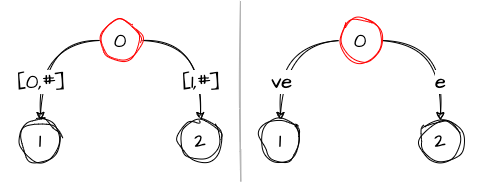
As in the previous step, the variables remain unchanged.

Step 3: vel

We do the same actions for the third character l:

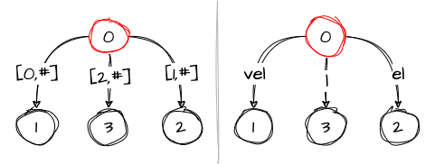
Again, no variables are modified.

Step 4: velv

Things get more interesting with the fourth character v. We already have it in the tree, represented by the edge vel, which leads to node 1. So instead of creating a new edge, we increment the remainder, set active_edge to the edge vel, and increase active_length to 1. This means that the active point now points from the root to the first character of the edge, which is the first v. The tree looks like this at this step, with # being 4:

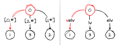
At this step, the variables have the following values:

remainder: 1
active_node: 0
active_edge: 'v'
active_length: 1

Step 5: velve

Things remain interesting in this step as well. First of all, the remainder is now 1, which means that in addition to the fifth character e, we should insert one more suffix, namely ve. However, we already have ve in the tree as part of the edge velve, so once again we increment the remainder and increase active_length to 2:

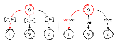
This leaves us with the modified variables:

remainder: 2
active_node: 0
active_edge: 'v'
active_length: 2

Starting from the next step, I’ll need more space for the illustrations, so I’ll only keep the visual representation of the tree on the right and not include the model representation on the left.

Step 6: velvet

Things get even more interesting here. The remainder is 2, which means that we should add three suffixes now: vet, et, and t.

Let’s start with vet by noticing that it is not in the tree. However, the active point points to the place where we should do the split and insert the suffix, which is the ve part of the velve edge. So we do the split. Then, according to rule 1, we should perform the following actions: keep the root as the active_node, set the active_edge to the first character of the next suffix (which is an edge that starts with e), and decrement the active_length:

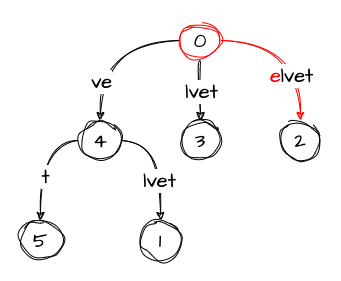
Since we dealt with the first of the suffixes in this step, we decrement the remainder as well. Just to recap, the variables now look as follows:

remainder: 1
active_node: 0
active_edge: 'e'
active_length: 1

Now, to the second suffix et. Again, we notice that it is not in the tree, which means we should do some splitting. The active point, pointing to the first e in the elvet edge, helps us find the split location. In addition to the split, we also should follow rule 2 and create a suffix link from the previously inserted node to the one we just created:

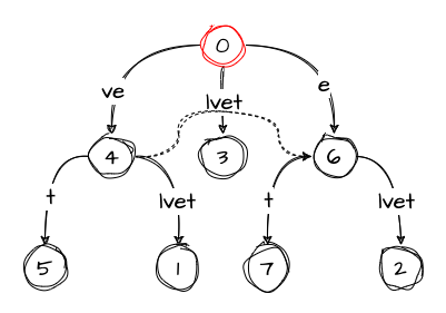
Since we did the split from the root, rule 1 also takes place. So the active_node remains the root, the active_edge is reset entirely because we don’t have an edge that starts with the next suffix t, and the active_length decreases down to 0. As with the previous suffix, we also decrement the remainder, so now it’s 0 as well.

Now we are back to the default values of the variables:

remainder: 0
active_node: 0
active_edge: ''
active_length: 0

But we still have one suffix left — t. Since we don’t have any edge that would have it, we just create a new node from the root:

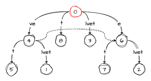
This time round we don’t need to change the variables.

Step 7: velvetv

Next, we move on to the character v in the string. We see that we already have an edge with this character, so we set the active point to point to that character and increase the value of the remainder:

remainder: 1
active_node: 0
active_edge: 'v'
active_length: 1

Step 8: velvetve

In this step, we again have the remainder telling us that we should insert two suffixes: ve and e. Since we have the entire ve edge already, we’ll do something interesting — we move the active point to node 4 and reset both active_edge and active_length:

Now we just need to increase the remainder:

remainder: 2
active_node: 4
active_edge: ''
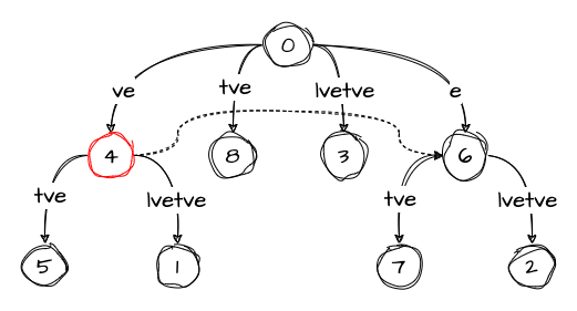
active_length: 0

Step 9: velvetvei

Moving on to the penultimate character i. At this moment, according to the value of remainder, we need to add three suffixes: vei, ei, and i.

We start by adding the suffix vei. Since we already followed the ve edge in the previous step, we insert a new node with an edge labeled i. As per rule 3, we also follow the suffix link from this node and set the active point to node 6:

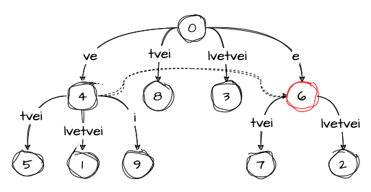
Don’t forget to decrement the remainder:

remainder: 1
active_node: 6
active_edge: ''
active_length: 0

The next suffix, ei, follows a similar path. We insert a new node with an edge labeled i. However, since there is no suffix link going out from this node, we reset the value of active_node to the root, as per rule 3. This brings us to the following state of the tree:

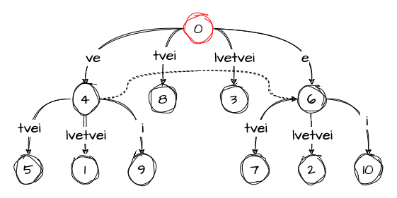
Since we alse decrement the remainder, we’re back to square one with the variables:

remainder: 0
active_node: 0
active_edge: ''
active_length: 0

Finally, since there is no i edge going from the root, we need to add a new node with such an edge to the tree:

The variables were not changed this time.

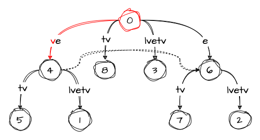
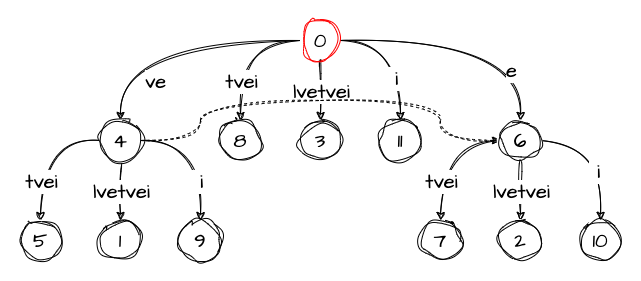
Step 10: velvetveil

The final step is similar to the ones where we processed a character that was already present in the tree. We just increase the value of remainder and set the active point to the edge containing the character:

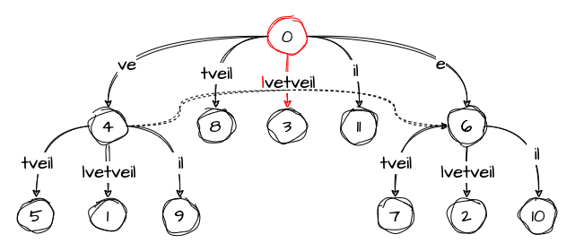
At the end of the algorithm, some variables have non-default values:

remainder: 1
active_node: 0
active_edge: 'l'
active_length: 1

But we, however, have all the suffixes added to tree in liniar time!

Implementation

Now let’s implement the algorithm in C#. Instead of starting from scratch, we will port a Java version that was posted in this Stack Overflow answer and slightly modify it for modern .NET.

To begin, we will combine the information for nodes and edges into a single class called Node:

internal class Node
{
  private readonly Dictionary<char, int> _children = new();

  internal int Start { get; set; }
  internal int End { get; }
  internal int SuffixLink { get; set; } = -1;

  internal Node(int start, int end)
  {
    Start = start;
    End = end;
  }
}

The Start and End properties contain an interval that marks a substring within the string. In the algorithm description, this information was held by edges. The SuffixLink property is a suffix link pointing to another node with the default value of -1, indicates that there is no suffix link going out from the node. Finally, _children represents the edges going out of the node. The char key indicates the direction and the int value holds the index of the node at the other end of the edge.

We also need a method for calculating an incoming edge’s length:

internal class Node
{
  // ...

  internal int EdgeLength(int position)
  {
    return Math.Min(End, position + 1) - Start;
  }
}

And a few methods for managing outgoing edges:

internal class Node
{
  // ...

  internal int this[char key] => _children[key];

  internal bool Contains(char key)
  {
    return _children.ContainsKey(key);
  }

  internal void Put(char key, int value)
  {
    _children[key] = value;
  }
}

The first one is an indexer for getting the right edge using the char key. Contains and Put are just wrappers around the Dictionary<TKey, TValue> class’ methods.

Next stop is NodeCollection, a custom container for holding Node instances:

internal class NodeCollection
{
  private readonly List<Node> _nodes = new();

  internal Node this[int index] => _nodes[index];

  internal int Add(Node node)
  {
    _nodes.Add(node);
    return _nodes.Count - 1;
  }
}

We could’ve used a standard List<T>, but we have a specific need for returning an index of the node that was just added, which is implemented by the Add method. We will see later why this is useful.

One final preparation is to create a struct called ActivePoint to manage the values of active_node, active_length, and active_edge:

internal struct ActivePoint
{
  internal int Node { get; set; }
  internal int Length { get; set; }
  internal int Edge { get; set; }
}

Construction

Now, to the class SuffixTree that has a big giant contructor in which we are going to implement Ukkonen’s algorithm:

public class SuffixTree
{
  private readonly NodeCollection _nodes = new();
  private readonly ReadOnlyMemory<char> _text;

  public SuffixTree(string line)
  {
    _text = line.AsMemory(); // (1)

    var root = _nodes.Add(new Node(-1, -1)); // (2)
    var activePoint = new ActivePoint();
    var remainder = 0;

    for (var i = 0; i < _text.Span.Length; i++) // (3)
    {
      var needSuffixLink = 0;
      remainder++;
      while (remainder > 0) // (4)
      {
        if (activePoint.Length == 0) activePoint.Edge = i; // (5)
        if (!_nodes[activePoint.Node].Contains(_text.Span[activePoint.Edge])) // (6)
        {
          var leaf = _nodes.Add(new Node(i, _text.Span.Length));
          _nodes[activePoint.Node].Put(_text.Span[activePoint.Edge], leaf);
          AddSuffixLink(activePoint.Node, ref needSuffixLink);
        }
        else // (7)
        {
          var next = _nodes[activePoint.Node][_text.Span[activePoint.Edge]];
          if (WalkDown(next, i, ref activePoint)) continue;

          if (_text.Span[_nodes[next].Start + activePoint.Length] == _text.Span[i])
          {
            activePoint.Length++;
            AddSuffixLink(activePoint.Node, ref needSuffixLink);
            break;
          }

          var split = _nodes.Add(new Node(_nodes[next].Start, _nodes[next].Start + activePoint.Length));
          _nodes[activePoint.Node].Put(_text.Span[activePoint.Edge], split);

          var leaf = _nodes.Add(new Node(i, _text.Span.Length));
          _nodes[split].Put(_text.Span[i], leaf);
          _nodes[next].Start += activePoint.Length;
          _nodes[split].Put(_text.Span[_nodes[next].Start], next);
          AddSuffixLink(split, ref needSuffixLink);
        }

        remainder--; // (8)

        if (activePoint.Node == root && activePoint.Length > 0) // (9)
        {
          activePoint.Length--;
          activePoint.Edge = i - remainder + 1;
        }
        else // (10) 
        {
          activePoint.Node = _nodes[activePoint.Node].SuffixLink > 0
            ? _nodes[activePoint.Node].SuffixLink
            : root;
        }
      }
    }
  }
}

This block of code may seem intimidating at first, but it is a straightforward implementation of the algorithm we discussed in the previous section. Let’s walkthrough its main parts:

1. We start by saving a reference to the source string text as a ReadOnlyMemory<char>. We actually need a Span<char>, but due to the stack-only nature of Span<T>, which introduces certain limitations, we have to use ReadOnlyMemory<char> instead. Essentially, it’s a wrapper around a Span<char> that helps mitigate some of the limitations, so we can use it as a class member.
2. Next, we initialize familiar variables that we will need later: root, activePoint, and remainder. Note that we initialize the root with -1s because it doesn’t hold any valuable information and only serves as a reference point.
3. We start the algorithm by going through each character of text one by one. For each character, we define a needSuffixLink variable setting it to 0 by default, and increment the remainder.
4. In the while loop, we go over the suffixes we need to add at each step, as the remainder tells us how many we have left.
5. In the first if statement, we check the current length of the active point: if it’s 0, we save the current character’s position as the active edge. Since we can exit the loop early, we might need the current step for calculating the positions of the suffixes correctly.
6. In the second if statement, we check if we have an edge that starts with the first character of the suffix. If not, we create a leaf and check if the active node needs a suffix link.
7. However, if the edge does start with the first character of the suffix, we have to perform a few actions:
   • First, we extract the node that the edge leads to, next, and check if we need to walk the edge to place the active point down the tree (we described that in the previous section). If so, we skip the rest of the steps and proceed to the next character of the suffix.
   • Otherwise, depending on the character, we either advance the active length or perform a split.
8. Don’t forget to decrement the remainder if we’re still here.
9. If the active node is the root, we have to decrement the active length and adjust the edge for the next suffix.
10. Otherwise, we follow the suffix link, if one is present.

AddSuffixLink has a simple implementation:

private void AddSuffixLink(int node, ref int needSuffixLink)
{
  if (needSuffixLink > 0)
  {
    _nodes[needSuffixLink].SuffixLink = node;
  }
  
  needSuffixLink = node;
}

WalkDown is not too hard either:

private bool WalkDown(int next, int position, ref ActivePoint activePoint)
{
  if (activePoint.Length < _nodes[next].EdgeLength(position)) return false;
  
  activePoint.Edge += _nodes[next].EdgeLength(position);
  activePoint.Length -= _nodes[next].EdgeLength(position);
  activePoint.Node = next;
  
  return true;
}

Search

Once the tree is defined, implementing a string searching algorithm that finds the first occurrence of a pattern will be easy:

public class SuffixTree
{
  // ...

  public int Search(string pattern)
  {
    if (pattern.Length > _text.Span.Length) return -1;

    var node = _nodes[0];
    var c = pattern[0];
    var patternIdx = 0;

    while (node.Contains(c))
    {
      var nodeIdx = node[c];
      node = _nodes[nodeIdx];
      for (var i = node.Start; i < node.End; i++)
      {
        if (_text.Span[i] == pattern[patternIdx]) patternIdx++;
        if (patternIdx == pattern.Length) return i - patternIdx + 1;
      }

      c = pattern[patternIdx];
    }

    return -1;
  }
}

To start, we traverse the tree from the root. We decide which outgoing edge to follow and check if the node contains a substring of the pattern using the Start and End properties. If it does, we continue walking down the tree by selecting the next edge. In the end, we either traverse all the characters that belong to the pattern and return the position of the first one, or return -1 to indicate that the pattern is not present in the source string.

Benchmarks

At the start of the post, it was mentioned that suffix trees can improve the performance of certain string search scenarios, like when we need to run multiple pattern searches on the same string. Let’s compare our implementation to the built-in IndexOf method, which is designed to find the first occurrence of a pattern and is optimized for vectorization.

In the benchmark, we will try to simulate a situation where we search for a short pattern multiple times on a string that contains 65,536 characters (which is not particularly large). We will use the same pattern for each search to make the benchmark more practical, as it would be tedious to use a unique pattern for each individual search. For this test, I will be using an Apple M1 chip:

• BenchmarkDotNet=v0.13.2, OS=macOS Monterey 12.6 (21G115) [Darwin 21.6.0]
• Apple M1 Pro, 1 CPU, 10 logical and 10 physical cores
• .NET SDK=7.0.101, .NET Runtime=7.0.1

|     Method |    N |          Mean |  Allocated |
|----------- |----- |--------------:|-----------:|
|    IndexOf |   1k |      7.896 ms |       13 B |
| SuffixTree |   1k |     22.414 ms | 15728056 B |
|    IndexOf |  10k |     78.900 ms |      117 B |
| SuffixTree |  10k |     22.915 ms | 15727880 B |
|    IndexOf | 100k |    789.086 ms |      816 B |
| SuffixTree | 100k |     29.227 ms | 15728366 B |
|    IndexOf |   1M |  7,880.230 ms |      816 B |
| SuffixTree |   1M |     92.972 ms | 15728628 B |
|    IndexOf |  10M | 78,805.910 ms |     1008 B |
| SuffixTree |  10M |    717.154 ms | 15728352 B |

As we can see, the time it takes for IndexOf to run is directly proportional to the number of searches N we perform on the string. The time it takes for a suffix tree search to run, on the other hand, increases somewhat logarithmically. However, it’s important to note that this improved performance comes at the cost of using more space to store the suffix tree.

For this benchmark, we used a fairly short pattern, but as the pattern gets longer, it takes more time for the algorithm to go through the tree. As the pattern size gets closer to the size of the source string, using a suffix tree becomes less practical. Which demonstrates the importance of testing performance for your specific cases.

You can check out the code from this post on GitHub: SuffixTreeSearch.

Further Reading

• Visualization of Ukkonen’s Algorithm
• Strings - Advanced data structures
• Suffix Tree using Ukkonen’s algorithm