The 24-Vertex Problem
If you’ve played FTL: Faster Than Light, a game described by its developer Subset Games as a “spaceship simulation roguelike-like”, you probably know it’s all about min-maxing. That is, maximizing your ship’s strengths and minimizing its weaknesses. It applies not only to the ship, though, as another strategy to a successful run is to explore a maximum number of beacons on the map before reaching the exit. It helps you collect more scrap (the in-game currency) and encounter events that could lead to various rewards. The game, however, plays against this strategy by introducing the Rebel fleet that advances through the map with each turn and limits your space for maneuvers:
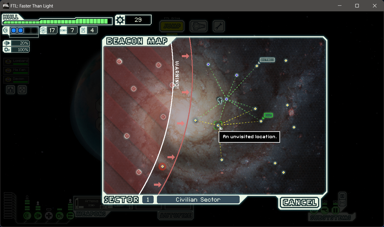
While it’s not an entirely bad idea to check out a beacon captured by the Rebels, it usually means facing a tough fight against their well-armed ship. Unfortunately, surviving the battle doesn’t come with any rewards. So, players often plan their route to the exit beacon, trying to avoid the Rebel fleet along the way.
This is where the game scratches my programming itch. Unfortunately, it’s likely impossible to create a program — let’s call it a navigator — that can visit all beacons just once, avoid Rebel-controlled ones, and exit before they catch up. Apart from the Rebels, there are other factors at play. Some beacons might be distress signals (like the one in the screenshot above) offering more rewards. Others could be stores the player wants to check out. Sometimes, it might be worth the risk to visit a Rebel-controlled beacon and jump to an interesting location from there. In certain situations, revisiting a beacon, which gives no reward, could be a strategic move. Finally, the game keeps beacon types a mystery until you land on a nearby one, so you don’t know which ones are worth checking out beforehand.
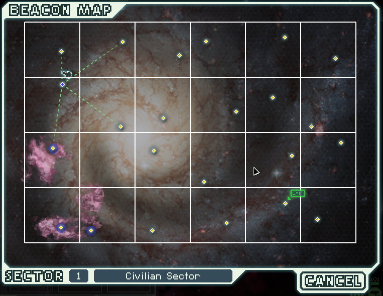
Now, let’s remove the fleet and different beacon types from the equation, and go back to the map again. The challenge of finding a path that starts from the beginning, reaches the exit, and covers as many beacons as possible remains interesting. For the rest of this post, we’ll work on making an FTL navigator that finds this path.
Problem
Let’s try to be a bit more formal and define the problem using math terms. As you may have noticed already, the map can be represented as an unweighted undirected graph1. That is, we only care if two vertices — since we talk proper math, it’s vertices now, not beacons — are connected or not. There is no associated weight or cost with the edge between them, and we can traverse the edge in both directions.
We will stay within game restrictions and say that the maximum number of vertices is capped at 24. Subset Games has posted an interesting tweet revealing how the beacon map is generated and where the 24 is coming from:
If you are familiar with graph theory, you probably see a resemblance between our problem and the Hamiltonian path problem. In the Hamiltonian path problem, we look for a path that visits every vertex in the graph exactly once, starting and ending at specific vertices.
We can think of our problem as a special case of the Hamiltonian path problem. The bad news is that it falls into the category of NP-complete problems, and therefore finding the solution may not be quick. The good news is that 24 vertices is a small enough problem space for a brute-force approach. However, it wouldn’t be a blog (mostly) about finding efficient solutions if we hadn’t explored a technique often used in NP-complete problems — dynamic programming. So, first we’ll solve our problem in a basic way using depth-first search, and then we’ll take a closer look at the Held-Karp algorithm and apply its variation.
Before we start coding, let’s define a graph that we are going to use throughout implementations as an input. We’ll use a Dictionary<int, HashSet<int>>, where the key is a vertex, and the value is a set of connected vertices. We use a HashSet<int> to take advantage of quick neighbor lookups since a vertex can’t have duplicate neighbors. A simple graph such as this one:

would be defined in C# as:
var graph = new Dictionary<int, HashSet<int>>
{
  [0] = new() { 1, 2 },
  [1] = new() { 0, 2, 3 },
  [2] = new() { 0, 1 },
  [3] = new() { 1 }
};
We also need to say which vertex we’re starting from (let’s call it start) and which one is the exit (end). The path we’re looking for will be a bunch of vertices, which we’ll represent as int[] in the code. So, in essence, we have to implement the following method:
int[] Solve(Dictionary<int, HashSet<int>> graph, int start, int end)Depth-First Search
Depth-First Search, or DFS for short, is a way to exhaustively go through each vertex in a graph until we reach the exit. We took a closer look at the algorithm in a previous post. The basic idea is to begin from the start, explore as far as possible on each branch before backtracking, and keep doing this until we’ve visited all possible vertices and reached the end. Here’s what we need to implement it:
- Begin with the
startvertex and mark it as visited. - Check an unvisited neighbor of the current vertex. If there is one, go to that neighbor and mark it as visited.
- Keep going, exploring as far as possible on each path.
- If there are no unvisited neighbors, backtrack to the previous vertex.
- Keep exploring until we reach the
end— and save it as a possible solution.
DFS naturally lends itself to exploring all paths to the end vertex before backtracking. In the end, we should pick the path with the most vertices.
Let’s put DFS into action. We’ll create two methods: Solve to set everything up and Dfs that’ll do the heavy lifting. First, let’s tackle Solve:
public static int[] Solve(Dictionary<int, int[]> graph, int start, int end)
{
  var solutions = new List<int[]>();
  var visited = new bool[graph.Count];
  var path = new Stack<int>();

  Dfs(graph, solutions, visited, path, start, end);

  return solutions
    .Aggregate((result, next) => result.Length > next.Length ? result : next)
    .Reverse()
    .ToArray();
}
Here, we make a List to hold all the possible solutions, each represented by int[]. We also create an array called visited to keep track of vertices visited by DFS. To track the current path DFS is going through, we need a stack named path.
We then use Dfs recursively to fill the solutions list with possible solutions. After DFS finishes its work, we pick the longest solution, reverse it (since it was stored in the stack), and return it to the caller.
Next, we implement Dfs by the book, with the only difference being that we save a path to solutions once we reach the end vertex:
private static void Dfs(
  Dictionary<int, int[]> graph,
  List<int[]> solutions,
  bool[] visited,
  Stack<int> path,
  int current,
  int end)
{
  visited[current] = true;
  path.Push(current);
  if (current == end)
  {
    solutions.Add(path.ToArray());
  }
  else
  {
    foreach (var neighbor in graph[current])
    {
      if (visited[neighbor]) continue;
      Dfs(graph, solutions, visited, path, neighbor, end);
    }
  }

  visited[current] = false;
  path.Pop();
}
The algorithm begins by marking the current vertex as visited and adding it to the stack. If this vertex turns out to be the end vertex, we’ve got a solution to save. If not, we check its neighbors: if we’ve been there before, we move on; if not, we run Dfs on them. When we’re done, we backtrack from the path by unmarking the current vertex as visited and removing it from the stack. That’s pretty much it.
But there’s a catch with DFS — it can be slow. In the worst case, there could be n! different sequences of vertices as potential Hamiltonian paths, where n is the number of vertices. This blows up into a factorial time complexity of O(n!). While we can certainly tweak DFS for some speed gains, it’s better to explore an alternative. Using dynamic programming, the Held-Karp algorithm can significantly speed up the process of finding the path.
Held–Karp Algorithm
The Held-Karp algorithm was initially made to solve the famous traveling salesman problem. But with a few tweaks, we can adapt it for our use. We’ll base our approach on an article by Clara Nguyễn and Natalie Bogda, Hamiltonian Paths & bitDP, where they applied the algorithm to a different variation of the Hamiltonian path problem. Even though they solve a slightly different problem, the main idea stays the same. So, we begin by following their path (no pun intended), but eventually, we’ll have to go our own way.
The main idea behind the Held-Karp algorithm is to use dynamic programming. This means we break the problem into smaller sub-problems and try to solve them instead. If that doesn’t work, we break those sub-problems into even simpler sub-sub-problems and keep going until we reach the simplest case we can handle. It might sound a lot like recursion, but there’s a twist. Recursion starts with the big problem and breaks it into smaller ones (top-down). Dynamic programming works the other way around; it solves the small sub-problems first, stores the result, and then uses it to solve the original problem (bottom-up).
Analysis
Let’s walk through the Held-Karp algorithm using the small graph we talked about earlier as an example. Our goal is to find a path from vertex 0 to vertex 3:
First, we list all different ways we can combine its vertices into subsets. For our graph, there are 16 possible combinations:
0000
0001
0010
0011
...
1111
Each subset shows which vertices are in it. For instance, the first subset has none, so it’s not useful for us. The second subset has only vertex 0, the third has only vertex 1, the fourth has both vertices 0 and 1, and so on. The last subset includes all the vertices of the graph. We can easily see that the total number of subsets is 2^n.
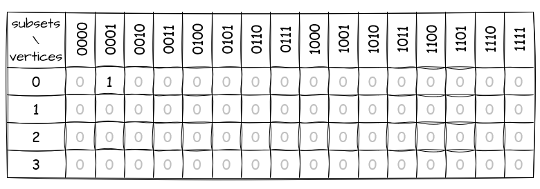
Now, we bring in something called the bitDP table (as named in Clara and Natalie’s article). This table keeps track of connections that lead from one subset of the graph to another. We’ll soon see how it helps us with our problem. For now, let’s start by filling the table with 0s:

The rows stand for the vertices, and the columns are the subsets.
Now, let’s fill in the table. First, we look for the subset that represents the starting vertex. In our graph example, that’s vertex 0, so the subset we’re looking for is 0001. We then put 1 in the cell that corresponds to vertex 0:
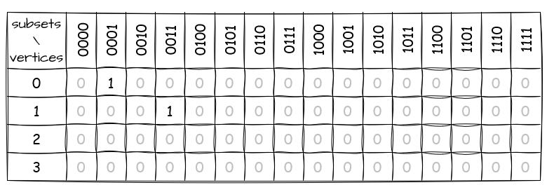
For the next step, we focus on the subsets that have two or more vertices: 0011, 0101, and so on. Here’s what we do: we take out one vertex at a time from a subset, and then we look at the new subset we’ve got. If any cells in the table have 1 for this new subset we’ve just made, we check if those vertices can connect to the one we’ve just taken out. If they can, we put 1 in the corresponding cell of the original subset. In practice, this means we can transition from one subset of the graph to another by connecting the vertices we marked with 1 to the vertex we removed from the subset.
Let’s process subset 0011 to illustrate this step:
- We take out vertices 0 and 1 individually, creating two new subsets:
0010and0001. - Checking
0010, we find no1s in the table, so nothing changes. This means there are no paths from vertex 0 in a subset with vertex 1 to a subset with both vertices 0 and 1. Which makes sense, as vertex 0 does not appear in the subset that only contains vertex 1. - Moving on to
0001, we go to its column. Here, only vertex 0 has1, and it can connect to vertex 1 in the graph. So, we update the table for0011by marking vertex 1 with1. This tells us there’s a path that connects vertices 0 and 1, leading from a subset with vertex 0 to a subset with both vertices 0 and 1.
Now the table looks like this:
We keep going through the same process for all the other subsets until we get to 1111. By that point, the table should look like this:
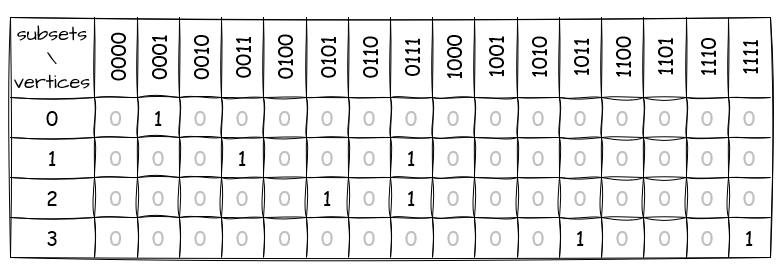
This table shows different sub-problems or sub-graphs, each being represented by a subset. Every column gives us information about the subset. If there’s a vertex marked with 1 in the column, it means there’s a path starting from vertex 0, going through all the vertices in that subset, and ending at the marked vertex. Pretty cool, right? It doesn’t show us the exact path, but we can figure it out by going through the table backward.
Start with the end vertex in the path, as we know it’s our last stop. Then, find a column that has at least one vertex marked with 1 and has as many vertices in the subset as possible. Notice how this connects with the original problem of “visit as many vertices as possible”? Now, we do the same we did for building the table, but in reverse order. Take out the end vertex from the subset, go to the resulting column, and see if there are any vertices marked with 1 that connect to the end vertex in the graph. If so, add it to the path, set the end vertex to the one we just found, and remove it from the subset, essentially moving to a smaller sub-problem. Repeat these steps until the subset has no vertices left.
Let’s use our graph example to see if we can find the path from vertex 0 to vertex 3:
- We start by adding vertex 3 to the path.
- Checking the table, we find a path from vertex 0 to vertex 3, covering all the vertices in the graph and having the end vertex set to
1, in column1111. We take out vertex 3 from it and move to0111. - At
0111, we have two cells marked with1. This means we can start from vertex 0, go through vertices 0, 1, and 2, and end up at either 1 or 2. Cool, but we need to get to 3 next. Consulting with the graph, we find that only vertex 1 connects to 3. So, we add vertex 1 to the path, consider it the new end, and remove it from the subset —0101. - Now at
0101, only vertex 2 is marked with1. We quickly check if 2 connects to the new end, 1. It does, so we add vertex 2 to the path, call it the new end, and remove it from the subset —0001. - Looking at
0001, we notice vertex 0 is marked with1. After making sure it connects to the new end, 2, we add it to the path, name it the new end, and remove it from the subset —0000. - Once we reach
0000, we stop moving through the table and look at what we have: [3, 1, 2, 0] — that’s the path, right? Not quite, because we need to reverse it: [0, 2, 1, 3] — there we go!
Two things we haven’t covered yet. First, what if we find many subsets that fit the conditions, having the same number of vertices and ending at the end one? This can happen in bigger graphs. But since, for our problem, the path’s exact look doesn’t matter as long as it has the maximum possible number of vertices, we just pick any subset. Second, when reconstructing the path, we might have a situation where two or more vertices go from one subset to another. This means the graph has more than one solution that visits the same vertices, but the path is different. Again, we just pick any of those vertices.
Now, let’s move on to how we write this algorithm in code.
Implementation
The main Solve method of the algorithm reflects what we discussed above. First, we make the bitDP table. Next, we find the subset with a path ending at the end vertex and the most vertices. Finally, we use the table to reconstruct the path:
public static int[] Solve(Dictionary<int, HashSet<int>> graph, int start, int end)
{
  var dp = CreateDp(graph, start);
  var subset = FindMaxSubset(dp, end);
  var path = ReconstructPath(graph, dp, subset, end);

  return path.ToArray();
}
Let’s tackle each part individually, starting by CreateDp:
private static bool[,] CreateDp(Dictionary<int, HashSet<int>> graph, int start)
{
  var n = 1 << graph.Count;
  var dp = new bool[n, graph.Count];
  dp[1 << start , start] = true;

  for (var i = 1 << start; i < n; i++) // (1)
  for (var j = 0; j < graph.Count; j++)
  {
    if (!CheckIfBitSet(i, j)) continue; // (2)
    var mask = ClearBit(i, j); // (3)
    for (var k = 0; k < graph.Count; k++)
    {
      if (!dp[mask, k] || !graph[k].Contains(j)) continue; // (4)
      dp[i, j] = true; // (5)
      break;
    }
  }

  return dp;
}
First off, we create the table. Since we only need 0s and 1s for the vertex cells, we use bool. There are 2^n columns, where n is the number of vertices in the graph, so we code column numbers as subsets. With integers that can hold up to 32 bits, we can easily handle subsets of 24 vertices and keep the array size safe. Then, we find the subset that has the vertex start and set its vertex value to true. Let’s now see how we fill in the table:
- We go through all the subsets, starting from
1 << startbecause we’re only interested in vertices connected tostart. So, we can skip processing the ones before it. - Next, we check each vertex in the subset and filter out the ones that don’t belong here.
- To take out each vertex individually, we XOR the subset against another one that contains only that vertex (since the subset is as an integer that can be seen as a bitmask, we just clear its
jth bit), giving us a new subset calledmask. - We look at the column
maskand check if any vertices are set totrueand if they connect to the one we just took out. - If we find any, we mark the processed vertex’s cell as
trueand move on to the next vertex from the subset.
I didn’t list code for CheckIfBitSet, ClearBit, and a few other methods that help with bit manupulations. You can find them in the repository linked at the end of the post.
Once we have the dp table created and filled, we call FindMaxSet:
private static int FindMaxSubset(bool[,] dp, int end)
{
  var maxSubset = 0; // (1)
  for (var i = 0; i < dp.GetLength(0); i++) // (2)
  {
    if (!CheckIfBitSet(i, end) ||
      !dp[i, end] ||
      CountBits(i) <= CountBits(maxSubset)) continue;
    maxSubset = i; // (3)
  }

  return maxSubset; // (4)
}
Our job here is to find the subset with the most vertices and where the end vertex is set to true. Here’s how we do it:
- We need a starting point, so we set
maxSubsetto0. - Going through all the subsets, we check:
- if they have the
endvertex - if that vertex is set to
true - if the number of vertices in the current subset is more than what we already found
- If all these conditions are met, we pick that subset as the new
maxSubset. - Once we’ve gone through all the subsets, we simply return
maxSubset.
Now that we have the subset, we can bring the path back using ReconstructPath:
private static Stack<int> ReconstructPath(Dictionary<int, HashSet<int>> graph, bool[,] dp, int subset, int end)
{
  var path = new Stack<int>(new[] { end }); // (1)
  while (subset > 0)
  {
    subset = ClearBit(subset, end); // (2)
    for (var j = 0; j < graph.Count; j++)
    {
      if (!dp[subset, j] || !graph[j].Contains(end)) continue; // (3)
      path.Push(j); // (4)
      end = j;
      break;
    }
  }

  return path;
}
This method looks a bit like CreateDp, but we’re moving backward from the end vertex to the start:
- We set up a stack to keep the
pathand put theendvertex in it right away because we know it should be there. - We go through each vertex in the subset, starting from the
end. But since we already added it to thepath, we take it out by clearing the bit that represents it and update thesubset. - We move to the new
subsetcolumn and check if there are any vertices marked astruethat lead to theend. - If we find at least one, we add it to the
path, update theendwith this vertex, and repeat the cycle until thesubsetis empty.
There you have it! The path is back in order.
Benchmarking
Sure, it’s tempting to compare two solutions and figure out which one is faster. But first, let’s think about two benchmark scenarios. One with graphs having 2, 4, 6, 8, and 10 vertices, where each vertex is connected to all others. And the other with a graph representing a real map from FTL.
I’ll run both benchmarks on the computer with the following specs:
- BenchmarkDotNet v0.13.10, Windows 11 (10.0.22631.2715/23H2/2023Update/SunValley3)
- Intel Core i7-10750H CPU 2.60GHz, 1 CPU, 12 logical and 6 physical cores
- .NET SDK 7.0.402, .NET Runtime=7.0.12
The results aren’t too surprising for graphs with lots of connections:
| Method | V  | Mean            | Error         | StdDev        | Allocated |
|------- |--- |----------------:|--------------:|--------------:|----------:|
| Dfs    |  2 |        137.0 ns |       2.75 ns |       2.95 ns |     344 B |
| Dp     |  2 |        141.4 ns |       2.72 ns |       2.27 ns |     208 B |
| Dfs    |  4 |        365.0 ns |       7.17 ns |      10.73 ns |     600 B |
| Dp     |  4 |      2,289.2 ns |      12.25 ns |      11.46 ns |     696 B |
| Dfs    |  6 |      3,914.2 ns |      75.35 ns |      97.97 ns |    5464 B |
| Dp     |  6 |      2,289.2 ns |      12.25 ns |      11.46 ns |     696 B |
| Dfs    |  8 |    132,324.6 ns |   2,370.23 ns |   2,217.11 ns |  138464 B |
| Dp     |  8 |     17,383.0 ns |     335.28 ns |     313.62 ns |    2368 B |
| Dfs    | 10 | 16,509,827.4 ns | 328,079.63 ns | 632,098.06 ns | 8863822 B |
| Dp     | 10 |     96,099.2 ns |   1,836.08 ns |   1,885.52 ns |   10656 B |
We can easily see Dfs’s factorial nature, while Dp grows exponentially. We probably can optimize DFS to allocate less memory and take early exits, but it won’t get significantly faster due to its asymptotic complexity. However, checking a real graph from the game with fewer edges might give us a surprising result:
| Method | V  | Mean        | Error     | StdDev    | Allocated |
|------- |--- |------------:|----------:|----------:|----------:|
| Dfs    | 24 |    81.22 ms |  1.408 ms |  1.622 ms |  22.01 MB |
| Dp     | 24 | 6,677.56 ms | 97.086 ms | 81.071 ms |    384 MB |
No surprises here, though. The performance of Dfs is heavily influenced by the number of connections between vertices. In contrast, for Dp, this number doesn’t matter much because it does the same operations regardless. There’s also room for tweaking Dp. For instance, we could pull some tricks to avoid checking certain vertices in the table. Or find a more efficient way to identify a subset with the maximum vertices. But, for this post, I’ll keep these optimizations out of scope.
Conclusion
The Held–Karp algorithm introduces an interesting tool, the bitDP table. In this post, we just explored one application of the table, but it can be handy for certain problems related to the Hamiltonian path problem. With it, we can quickly figure out the number of paths going through all vertices by checking the last column and counting vertices marked as 1. We can also count the number of Hamiltonian cycles or reconstruct the shortest path between the starting and ending vertices.
You can check out the code from this post on GitHub: FtlNavigator.
Multiverse, an FTL mod that adds a lot of new content to the base game, actually shows the beacon map as a graph. ↩︎