May 5, 2022

Programming Guitar Music

go audio processing fun

In this blog, I usually write about approaches and technologies that help us build more efficient software. But this time round we’re going to do something different. We’ll talk about sound waves, learn how they’re stored in computers, simulate a guitar string sound, and perform a cover of Johnny Cash’s version of Hurt — in a geeky way. So we won’t use any pre-recorded samples, sequencers, or — heaven forbid — actual guitars. Instead, we will employ a little bit of math, Go, and a few helper libraries for audio processing.

But first, let’s dive into the underlying theory. We won’t be talking about the physics of sound waves and all the rest of it, but only glance over some concepts to establish common ground we’re going to build our code upon.

Sound in Computers

In physics, sound is a complex phenomenon that involves propagation of acoustic waves, pressure compressions and rarefactions, and many other things. When it comes to representing sound visually, it can often be depicted as a wave:

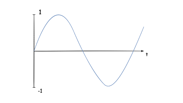
The wave, in turn, can also be interpreted as a function of time that outputs values between -1 and 1. The wave has a lot of characteristics, but in the context of this post, we are only interested in two: length and frequency. The former is rather intuitive, that’s just how long the wave is, measured in time units, like seconds or minutes. The latter, though, describes a repetition of the waveform. For example, the frequency of the yellow wave is twice that of the blue one:

To measure a wave’s frequency, we need to count the number of waveform repetitions in one second. If we only have one waveform that spans through the second, the wave’s frequency would be one hertz or 1 Hz. It would be impossible to hear, though, as humans can only detect sounds in a frequency range from 20 Hz to 20 kHz.

The waves in the pictures above are analog, as each is represented by a continuous function, i.e. we can obtain a function value at every moment in time. Well, it creates a problem, because as time is continuous we would have to store an infinite amount of numbers on a computer that has finite space. The answer to this conundrum is sampling: we convert our continuous wave into a series of function values measured at a specific time interval. The values we get are called samples. Depending on the time interval, the conversion might produce different numbers of samples, for example, this:

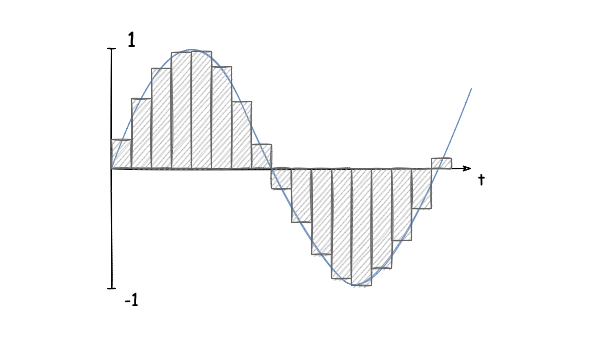
Or this one:

Of course, the more samples we have, the more precise the sound would be. Sampling is also measured in hertz, and it’s referring to how many samples we have in one second — this measurement is called the sample rate. A common sample rate used in audio processing, that we’re also going to use throughout the post, is 44,100 Hz.

Now that we have familiarized ourselves with a little bit of theory, let’s create a sound. We start with the basic wave, a sine wave, which can be described like that:

Where f is angular frequency, n is our samples, and y(n) is the wave we are after.

Let’s write some code to synthesize sound:

const SampleRate = 44100

func Synthesize(frequency float64, duration float64) []float64 {
  size := duration * SampleRate
  samples := make([]float64, size)
  for i := range samples {
    samples[i] = math.Sin(2 *math.Pi * frequency * float64(i) / float64(size))
  }

  return samples
}

This is just one example of how we could generate a sound wave in Go, but it will do. First, we set the size, or the number of samples in our wave, using duration in seconds and SampleRate. Then we create our output slice of samples. Finally, we use the formula to compute each sample.

We will come to the method that records sound a bit later. For now, let’s just pass to the function 329.63 Hz as frequency (that’s the frequency of the E4 note, the first string on a guitar), and 4 seconds as duration, and see — or rather hear — what we get:

Well, that’s surely something, but it doesn’t sound particularly pleasant. Luckily, we have an interesting algorithm which would make the same tune sound as it was played on a guitar.

Karplus-Strong Algorithm

The Karplus-Strong algorithm described in this article allows us to synthesize a sound that closely resembles a plucked guitar string. Again, we won’t go into the nitty-gritty details of how it works, but rather explore the algorithm’s components and try to implement it. Let’s have a look at the diagram:

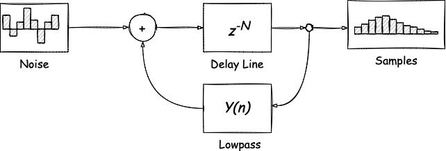
What happens here is the following:

1. We generate a short array of noise, that is, an array of random numbers. Its size is directly connected to the sound’s frequency, as it should be calculated as SampleRate / frequency.
2. We pass the noise array through a delay line, effectively producing new samples. The delay line is a component that models sound’s propagation delay.
3. We apply a lowpass filter to pass low-frequency values and impede high-frequency values, making the sound more muffled and smooth.

The delay line is fairly easy to express:

Where N is the size of the noise array. There are many variations of a lowpass filter, but we are going to use the one defined in the article:

We can code the algorithm like this:

func Synthesize(frequency float64, duration float64) []float64 {
  noise := make([]float64, int(SampleRate/frequency))
  for i := range noise {
    noise[i] = rand.Float64()*2 - 1
  }

  samples := make([]float64, int(SampleRate*duration))
  for i := range noise {
    samples[i] = noise[i]
  }

  for i := len(noise); i < len(samples); i++ {
    samples[i] = (samples[i-len(noise)] + samples[i-len(noise)+1]) / 2
  }

  return samples
}

First, we create a slice of random numbers noise. Then we create our output and fill in the first samples with the noise. The rest of the samples are calculated according to the formula, but we have to shift noise to take the delay line into account, that’s why we subtract len(noise) in the calculations.

Let’s try the same first string:

Sounds better, huh? What about the sixth string:

We can play with the algorithm trying to find a better tune, but I suggest we move forward and explore the extended version.

Extended Karplus-Strong Algorithm

To implement the extended Karplus-Strong algorithm, or EKS for short, we are going to closely follow this article describing the algorithm in detail. It’s a bit heavy on math, but it would give us more control over the output sound. Let’s start with the diagram:

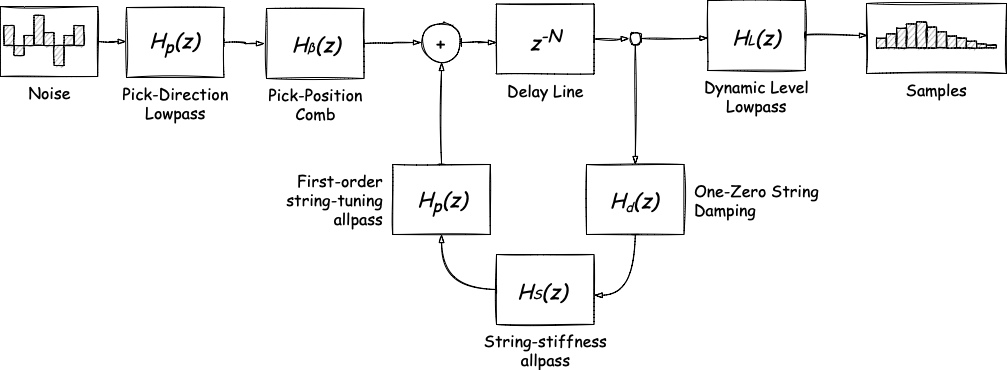
The core idea is somewhat similar to the basic Karplus-Strong: we make some noise in the beginning, then we generate sound somewhere in the middle, and we get final samples. Unlike its predecessor, though, EKS’s middle part goes up to eleven as we have different filter groups, each of which applies to different parts of the pipeline. We can define the groups like that:

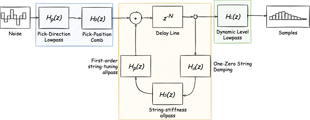
The blue one is responsible for noise generation and applying noise filters. The yellow group generates new samples and processes each sample individually, passing it through a set of single sample filters. Finally, the green one applies all samples filters before output. One of the main ideas of the extended algorithm is that we can mix and match different filters within each group.

Before we break the filters down, let’s briefly take a slight detour and make a note of the Z-transform each filter is based upon. In a general form, the Z-transform can be written as:

Without diving too deep into the math, let’s say that this formula can be expanded as:

Where x is an input array and y is an output array. The Z-transform has an important feature that we should take into account: for each out-of-range n the result of the function is 0, that is, x(-1) = 0. Now, to the filters.

Noise Filters

We start with the pick-direction lowpass filter, which, as the name implies, is responsible for the pick direction, as “up-pick” and “down-pick” have different coefficients. The Z-transform for the filter is:

It can be expanded into the formula:

Coefficient p affecting the direction has a constraint: 0 <= p <= 0.9. For simplicity, we are going to use value 0.9 indicating downward picking. We can express this filter in code like this:

const p = 0.9

func pickDirectionLowpass(noise []float64) {
  buffer := make([]float64, len(noise))
  buffer[0] = (1 - p) * noise[0]
  for i := 1; i < len(noise); i++ {
    buffer[i] = (1-p)*noise[i] + p*buffer[i-1]
  }
  noise = buffer
}

First, we create a buffer slice of the same size as the incoming noise. Next, we initialize its first element as (1 - p) * noise[0] since the second term in the formula is going to be 0 (remember that according to the Z-transform p * buffer[-1] would give as 0). Then we apply the formula to the rest of the noise slice. Finally, we assign the buffer to noise.

The second filter in this group is the pick-position comb filter that determines the position at which the string was picked:

The expanded version of the formula:

Coefficient β which has a constraint 0 <= β <= 1 is responsible for the pick position. We will be using value 0.1 indicating picking near the guitar’s sound hole. The bigger the value, the further away from the sound hole picking is. The filter would be represented in code as another function:

const b = 0.1

func pickPositionComb(noise []float64) {
  pick := int(b*float64(len(noise)) + 0.5)
  if pick == 0 {
    pick = len(noise)
  }
  buffer := make([]float64, len(noise))
  for i := range noise {
    if i-pick < 0 {
      buffer[i] = noise[i]
    } else {
      buffer[i] = noise[i] - noise[i-pick]
    }
  }
  noise = buffer
}

We just calculate the pick value and apply the formula. One thing to note here: if pick ends up being rounded to zero by the integer conversion, we would assign pick value to the size of noise, effectively turning the filter off.

Single Sample Filters

Following arrows on the diagram, we start exploring single sample filters with the delay line, which generates new samples and has probably the simplest formula:

Translating to something familiar as we were using the same delay line formula in the basic Karplus-Strong:

Where N is the size of the noise array. Keeping in mind possible out-of-range values, we can implement the delay line like that:

func delayLine(samples []float64, n, N int) float64 {
  if n-N < 0 {
    return 0
  }
  return samples[n-N]
}

One thing to note before we go further: in this filter group, each filter needs access to samples to get a previous sample and to N to shift the noise array, so all filter functions should have the same signature. Also, each filter’s output is the next filter’s input, so starting from the second filter we should include a call to the previous one.

Next in this group is the one-zero string damping filter, which has an effect on string decay:

The formula can be rewritten as:

S is called the stretching factor and has a constraint: 0 <= S <= 1. If S equals to 0 or 1 there won’t be any decay. We are going to use 0.5 as the stretching factor to obtain the fastest decay. This one is also easy to express in code:

const s = 0.5 

func oneZeroStringDamping(samples []float64, n, N int) float64 {
  return (1-s)*delayLine(samples, n, N) + s*delayLine(samples, n-1, N)
}

Then we have the string-stiffness allpass filter on the list. To be honest, I could not find a way to expand its Z-transform into a more useful form we could work with:

There’s a description of the filter, but I don’t think my math skills are on par with it. Please do let me know if you happen to puzzle this out. Meanwhile, we skip this particular filter and see if it affects the output (spoiler: the output still sounds good).

The fourth and the final filter in this group is the first-order string tuning allpass filter, which has the following Z-transform:

In other words,

Where C is the coefficient affecting the string delay that has a constraint -1 <= C <= 1. Again, this filter is not too hard to code:

const c = 0.1

func firstOrderStringTuningAllpass(samples []float64, n, N int) float64 {
  return c*(oneZeroStringDamping(samples, n, N)-samples[n-1]) + oneZeroStringDamping(samples, n-1, N)
}

All Samples Filters

Finally, the all samples filter group that only contains the dynamic level lowpass filter:

Which actually has two expanded formulas that we have to use one after another. First formula:

In which w can be calculated as:

Where f is frequency and Fs is the sample rate. Second formula:

Where coefficient L affects the level, or the volume, of the samples and has the constraint 0 <= L <= 1. At the maximum value 1 the filter is bypassed. We are going to use level 0.1 in code:

const l = 0.1

func dynamicLevelLowpass(samples []float64, w float64) {
  buffer := make([]float64, len(samples))
  buffer[0] = w / (1 + w) * samples[0]
  for i := 1; i < len(samples); i++ {
    buffer[i] = w/(1+w)*(samples[i]+samples[i-1]) + (1-w)/(1+w)*buffer[i-1]
  }

  for i := range samples {
    samples[i] = (math.Pow(l, 4/3) * samples[i]) + (1-l)*buffer[i]
  }
}

Just for convenience, we compute w in the caller code and pass it down to the function. Here we again create a buffer for storing filtered samples. Then we apply the first formula to the first buffer element manually (keeping in mind that the second term in the formula would give us 0 due to the negative index). Next, we apply the first formula to the rest of the buffer. Finally, we apply the second formula to all samples.

Putting It All Together

Now, that all filters are done, we can finally implement the whole algorithm:

func Synthesize(frequency float64, duration float64) []float64 {
  noise := make([]float64, int(SampleRate/frequency))
  for i := range noise {
    noise[i] = rand.Float64()*2 - 1
  }

  pickDirectionLowpass(noise)
  pickPositionComb(noise)

  samples := make([]float64, int(SampleRate*duration))
  for i := range noise {
    samples[i] = noise[i]
  }

  for i := len(noise); i < len(samples); i++ {
    samples[i] = firstOrderStringTuningAllpass(samples, i, len(noise))
  }

  dynamicLevelLowpass(samples, math.Pi*frequency/SampleRate)

  return samples

First, we create a slice containing initial noise, exactly as we did in the basic version of Karplus-Strong. Then we pass it down to the noise-applied filters. Next, we create samples and add some noise in the beginning. Then we run our sample-based filters on each sample. Finally, we pass the samples through the dynamic level lowpass filter.

Let’s now hear the result. Open first string:

Sixth string:

By changing the constants we defined along the way, we could hear how they affect the output sound.

Sound in Go

Now that we know how to produce sound, we can create a few abstractions to play and record it. But first, let’s make a note — I mean, a musical note. Since the note is just a frequency value, like 329.63 Hz for note E4 (remember that’s the first guitar string), we could define it as a float. However, we are going to model a guitar, so we go full guitar mode and define a note as a combination of a string and fret. That is, note E4 would be written as {1, 0} meaning the first string with no fret clamped. In code that would be a struct:

type Note struct {
  String int
  Fret   int
}

In order to fetch the correct frequency value, we have to put a big giant map that takes a note and returns frequency somewhere in code:

var frequencies = map[Note]float64{
  Note{1, 0}:  329.63,
  Note{1, 1}:  349.23,
  // ...
  Note{6, 19}: 246.94,
}

Just for our convenience, we can also decouple the way we synthesize sound from the rest of the application by introducing the synthesizer interface. So we can plug in either basic or extended Karplus-Strong implementations, or any other algorithm that satisfies the interface:

type synthesizer interface {
  Synthesize(frequency float64, duration float64) []float64
}

Once we defined a note and synthesizer, we can move on to playing and recording. To manipulate sound in Go, we are going to use a package called beep. This package provides ways to control, transform, and transfer sound data. The core abstraction all these actions use is the Streamer interface, which is somewhat similar to io.Reader, but for audio:

type Streamer interface {
  Stream(samples [][2]float64) (int, bool)
  Err() error
}

Stream takes samples in and returns a number of streamed samples and whether it’s reached the end. samples is a streaming buffer for the left and right channels, that’s why its type is [][2]float64. As the name implies, Err just signals if there was an error in streaming.

Since we are working with a buffer, we need to store the total number of generated samples and the number of processed samples — struct sound would be a good place for it:

type sound struct {
  totalSamples []float64
  processed    int
}

func newSound(synth synthesizer, note Note, duration float64) *sound {
  return &sound{synth.Synthesize(frequencies[note], duration), 0}
}

To make it more convenient for the caller, we defined the sound constructor as well. In it, we automatically call Synthesize to generate the samples and set 0 as the number of processed samples. Now, to make sound streamable, we have to implement the Stream and Err methods:

func (s *sound) Stream(samples [][2]float64) (int, bool) {
  if s.processed >= len(s.totalSamples) {
    return 0, false
  }

  if len(s.totalSamples)-s.processed < len(samples) {
    samples = samples[:len(s.totalSamples)-s.processed]
  }

  for i := range samples {
    samples[i][0] = s.totalSamples[s.processed+i]
    samples[i][1] = s.totalSamples[s.processed+i]
  }

  s.processed += len(samples)

  return len(samples), true
}

func (s *sound) Err() error {
  return nil
}

The Stream implementation is fairly simple, but we have to keep an eye on the number of samples left in the buffer and signal with 0, false once we reach the end. As for Err, we do not expect any errors during streaming (I bet that would be my famous last words). Now we can use some interesting beep methods, passing around our sound struct.

Modeling a Guitar

Okay, we are just one struct away from playing and recording sound. We also came closer to the post title, making guitar music. Not surprisingly, a guitar would be yet another struct:

type Guitar struct {
  synth synthesizer
}

func NewGuitar(synth synthesizer) *Guitar {
  return &Guitar{synth}
}

Experienced guitar players could extract sound in numerous different ways, but in this post we only need two: pluck and chord.

func (g *Guitar) Pluck(note Note, duration float64) beep.Streamer {
  return newSound(g.synth, note, duration)
}

func (g *Guitar) Chord(notes []Note, duration, delay float64) beep.Streamer {
  streamers := make([]beep.Streamer, len(notes))
  for i, note := range notes {
    silence := beep.Silence(int(SampleRate * delay * float64(i)))
    sound := newSound(g.synth, note, duration-delay*float64(i))
    streamers[i] = beep.Seq(silence, sound)
  }

  return beep.Mix(streamers...)
}

Pluck is simple as it’s just a sound wrapper. Chord, on the other hand, is way more interesting. As a guitar chord is just a set of strings being plucked (almost) at the same time, we can model it as a slice of Streamers, each of which is represented by sound. Now, every string starting from the second one is plucked with a slight delay, hence we need to add increasing silence before each pluck and address sound duration accordingly. We can add delays using beep.Silence, which is also a Streamer, and combine two streamers together with beep.Seq. Once all streamers are added to the resulting slice, we pass it to beep.Mix, effectively producing a new streamer that would play them all at the same time. Example of a C-chord:

Chord has an interesting property. If delay was zero, the chord would sound like a set of notes played at the same time as in fingerstyle, like this:

The bigger delay gets, the more it sounds like a broken chord. Once delay hits value duration / len(notes) it becomes arpeggio:

Last but not least, sometimes we need to make pauses in melody, so we add this convenient method to the guitar:

func (g *Guitar) Silence(duration float64) beep.Streamer {
  return beep.Silence(int(g.sampleRate * duration))
}

Which is, again, just a wrapper around beep.Silence. Now we can mix and match plucks and chords with beep.Seq and beep.Mix to produce and play music:

kse := karplusstrong.NewExtended()
guitar := guitar.NewGuitar(kse)

music := beep.Seq(
  g.Pluck(guitar.Note{1, 0}),
  g.Chord([]guitar.Note{ {5, 3}, {4, 2} }, 1, 0.25),
)

speaker.Play(music)

Or record it to a file:

f, _ := os.Create("music.wav")
defer f.Close()

format := beep.Format{SampleRate: SampleRate, NumChannels: 2, Precision: 2}
wav.Encode(f, g.Pluck(guitar.Note{1, 0}), format)

It would be strange to assemble a guitar literally from scratch and to put it in the corner, wouldn’t it? Let’s perform a small portion of Johnny Cash’s version of Hurt¹:

Conclusion

I know, I know, this “guitar” barely reaches a MIDI level, but hey, we just synthesized its sound literally out of nowhere. Besides, this rendition is performed by a soulless machine, we gotta respect our future overlords cut it some slack! On a more serious note, I think using generative algorithms might help find suitable constants for improving the synthesis and making it sound more real. But that’s a story for another time.

Many thanks to Daiwery for the initial research² and inspiration and to Tero Nurmiluoto for a very thorough review.

You can check out the code from this post on GitHub: music.

Further Reading

• Music and Computers
• Creating sound from scratch with Go
• Extensions of the Karplus-Strong Plucked-String Algorithm

Footnotes