Computing the Convex Hull on GPU
We have talked about hardware acceleration in one of the previous posts where we briefly touched upon the topic of CPU-specific instructions and, in particular, SIMD usage. However, the CPU is not the only piece of hardware programmers can use for computations. Modern desktop computers and some servers are often equipped with graphics cards. Their primary purpose was to render graphics, which, as a side-effect, made them excellent for the computation of complex and high-volume matrix mathematics.
General-purpose computing on GPUs began to appear in the early 2000s. Back then it was difficult to translate programming concepts into graphics terms. However, later on, graphics card manufacturers introduced special interfaces for general-purpose programming, like OpenCL and CUDA.
On the GPU, programmers can execute code on multiple device cores in parallel. Modern graphics cards are designed to run thousands of threads. They also offer higher memory bandwidth and instruction throughput than CPUs. A common GPU programming pattern is to prepare data on the CPU side, copy it to the graphics card’s memory, process data there, and copy results back for future use. Of course, there is an overhead due to additional complexity and copying data back and forth, but parallelization can make up for it on large input.
GPU programming is different from what we are used to on the x86 platform. It implies programming in the SIMT paradigm, meaning we run a single instruction on multiple threads, which is akin to SIMD, where we store multiple data in CPU registers and then process it with a single instruction. When relying on CPU acceleration we often need to refactor only some parts of our code using more or less the same x86 instructions. In GPU programming, on the other hand, the platform is different, and so are the instructions. That often implies significant changes to the code we want to accelerate.
GPU programming has its drawbacks. Aside from code changes mentioned above, one of the main problems is, perhaps, portability. Even within a single graphics card manufacturer the same code that runs perfectly on one device might crash on the other due to less memory or a different API version.
In this post, I will be talking about and working with the CUDA platform, for that reason I’ll use Nvidia’s terminology.
CUDA Programming Model
CUDA, or Compute Unified Device Architecture, is a computing platform created by Nvidia. It provides an easy way to program on CUDA-supported GPUs. Even though Nvidia explains how to write applications using the platform in CUDA C++ Programming Guide, I’ll briefly mention some essentials before we go further.
In Nvidia terms, code that’s supposed to run on the GPU is called device code as opposed to host code that (you guessed it) runs on the CPU. Similarly, there are device memory and host memory.
Device code is usually broken down into kernel functions that the host calls when GPU power is needed. CUDA organizes threads into blocks and then blocks into a grid. When a kernel is executed, the whole grid is assigned to the job. Block size can be defined to some extent, although there is a limit. Modern GPUs can contain up to 1024 threads per block.
Kernels are typically run in parallel by multiple GPU threads, one thread per data element in most cases. Threads can also synchronize with each other within the same block.
We can outline the following hierarchy of the programming model:
Grid
-- Block 0
---- Thread 0
---- Thread 1
---- ...
---- Thread N
-- Block 1
---- Thread 0
---- Thread 1
---- ...
---- Thread N
...
-- Block M
---- Thread 0
---- Thread 1
---- ...
---- Thread N
Internally, CUDA runs 32 threads at the same time by grouping them together into something that’s called a warp. In a typical scenario, the block size is a multiple of the warp size.
GPUs normally have multiple streaming multiprocessors (SMs), each containing numerous CUDA cores as well as cache and memory that are shared between the cores. When calling a kernel function CUDA assigns one block to one SM. It might be so that there are more blocks than SMs, therefore some of them have to wait. Once an SM finishes block processing, another block is scheduled.
Here is how the programming model maps to the hardware description:
Grid   -> GPU
Block  -> SM
Thread -> Core
The CUDA toolkit comes with the NVCC compiler that allows C/C++ programs to use CUDA syntax extensions. NVCC statically links the program with the CUDA runtime library. However, a C/C++ program can also dynamically link the runtime library and ship it along.
To see how it all works, let’s borrow a slightly modified simple CUDA program from Nvidia’s blog post An Even Easier Introduction to CUDA. The program just sums up two arrays of floats:
int main(void) {
  int N = 1000000;
  float *x, *y;

  cudaMallocManaged(&x, N * sizeof(float));
  cudaMallocManaged(&y, N * sizeof(float));

  for (int i = 0; i < N; i++) {
    x[i] = 1.0f;
    y[i] = 2.0f;
  }

  int blockSize = 256;
  int numBlocks = (N + blockSize - 1) / blockSize;
  add << <numBlocks, blockSize >> > (N, x, y);
  cudaDeviceSynchronize();

  float maxError = 0.0f;
  for (int i = 0; i < N; i++) {
    maxError = fmax(maxError, fabs(y[i] - 3.0f));
  }

  std::cout << "Max error: " << maxError << std::endl;

  cudaFree(x);
  cudaFree(y);

  return 0;
}

__global__ void add(int n, float *x, float *y) {
  int index = blockIdx.x * blockDim.x + threadIdx.x;
  if (index > n) return;

  y[index] = x[index] + y[index];
}
Let’s break the program down starting from the main function.
First, we set N as the number of elements for both arrays, x and y.
Then cudaMallocManaged tells CUDA to allocate something that’s called Unified Memory. Since we have two kinds of memory, on the device and on the host, we have to copy data from one to the other depending on where we need it. Unified Memory does it for us by creating a pool of managed memory behind the scenes, migrating data between device and host, and providing a single pointer to access both. Once memory is allocated, we initialize the arrays.
Next, we set blockSize (the number of threads in a block) and compute numBlocks (the number of blocks in a grid). Based on 256 threads and 1 million elements we should get 3907 blocks.
We run the kernel function add providing blockSize and numBlock with a special triple bracket syntax and passing array pointers along with the number of their elements.
The kernel add is defined below with a special keyword __global__. In the function, we need to figure out the index of the current element. We can calculate it using built-in blockIdx, blockDim, and threadIdx variables that give us the block index, block size, and thread index within the block, respectively. While CUDA supports 1D, 2D, 3D data — vector, matrix, and volume (a 3D array) — in this post we work with vectors, therefore we only access x property when computing the index.
It’s worth mentioning that we are working with the array of 1 million elements, hence we have to ignore every index that goes beyond its length. Due to the warp size, CUDA might spawn more threads than we have elements if we don’t align our data.
Finally, we wait for the GPU to finish its job, check that we get the results we were waiting for, and free the memory. The output of the function is:
Max error: 0ILGPU
As a developer who works with C# and .NET on an everyday basis, I was tempted to try GPU programming in a familiar environment. However, it’s not that simple in the .NET land. We don’t have a runtime library that could help us incorporate GPU code into C#. Not to mention that unlike C++ .NET doesn’t compile C# code directly into machine code. Instead, it converts the source code to the intermediate language (IL) producing .exe or .dll files. Then the .NET runtime uses Just-In-Time (JIT) compiler to convert the IL to the machine code.
Luckily, there are a couple of options that come to the rescue. I decided to go with the one that’s open-source, free, and (in my opinion) easy to use — ILGPU. ILGPU is a JIT compiler that can translate the IL into code running on the GPU.
We won’t dive into details of how ILGPU works, instead, we’ll use it and port the C++ program above to C# and see what happens:
private static void Main()
{
  const int n = 1_000_000;

  using var context = new Context();
  using var accelerator = new CudaAccelerator(context);
  using var x = accelerator.AllocateExchangeBuffer<float>(n);
  using var y = accelerator.AllocateExchangeBuffer<float>(n);

  for (var i = 0; i < n; i++)
  {
    x[i] = 1.0f;
    y[i] = 2.0f;
  }

  x.CopyToAccelerator();
  y.CopyToAccelerator();
  accelerator.Synchronize();

  var blockSize = 256;
  var numBlocks = (n + blockSize - 1) / blockSize;

  var addKernel = accelerator.LoadStreamKernel<int, ArrayView<float>, ArrayView<float>>(AddKernel);
  addKernel(new KernelConfig(numBlocks, blockSize), n, x.View, y.View);
  accelerator.Synchronize();

  y.CopyFromAccelerator();
  accelerator.Synchronize();

  var maxError = 0.0f;
  for (var i = 0; i < n; i++)
  {
    maxError = Math.Max(maxError, Math.Abs(y[i] - 3.0f));
  }

  Console.WriteLine($"Max error: {maxError}");
}

private static void AddKernel(int n, ArrayView<float> xView, ArrayView<float> yView)
{
  var index = Grid.GlobalIndex.X;
  if (index > n) return;

  yView[index] = yView[index] + xView[index];
}
The program works the same way as its C++ equivalent but with some additional details.
First, we have to create instances of Context and CudaAccelerator through which we will interact with the GPU.
ILGPU provides us with ExchangeBuffer<T> which is somewhat similar to how Unified Memory works in the C++ example. Using a buffer created both in device memory and host memory, we can copy data between device and host by calling CopyToAccelerator() and CopyFromAccelerator on the accelerator instance. We also need to wait for the GPU to do the copying by calling Synchronize().
Once the buffers x and y are allocated, we need to initialize them.
Similarly to C++, we calculate blockSize and numBlocks. It seems that ILGPU uses the word “group” for the CUDA term “block”. I assume this is due to its working not only with CUDA but with other accelerators as well.
The next step is to load the kernel function, providing blockSize and numBlocks as the kernel configuration. The kernel looks quite the same, except we don’t need to calculate an index by hand. ILGPU does it for us providing the static Grid.GlobalIndex.X property.
Finally, we wait for the GPU to complete the task, copy data back to the host, and check the results. The output should be the same as in the C++ program:
Max error: 0Doesn’t look very difficult, does it?
Summing arrays is surely fun, but let me pick a (more or less) real problem and throw it onto the GPU. Following this hands-on approach, we can explore more ILGPU features.
Problem
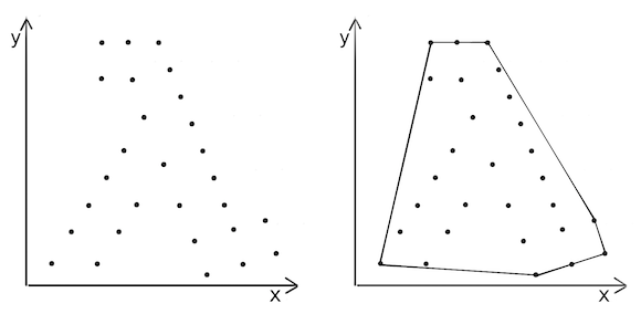
This time round we will solve the convex hull problem from the computational geometry field. What we need to do is to compute the convex hull based on a set of points in a two-dimensional space. That is, given points on the left we should draw a polygon on the right:
Quickhull
To achieve this goal we will use the Quickhull algorithm. In a way, it resembles well-known Quicksort because of its divide and conquer nature, but works on a 2D space rather than on an array.
Quickhull is fairly simple:
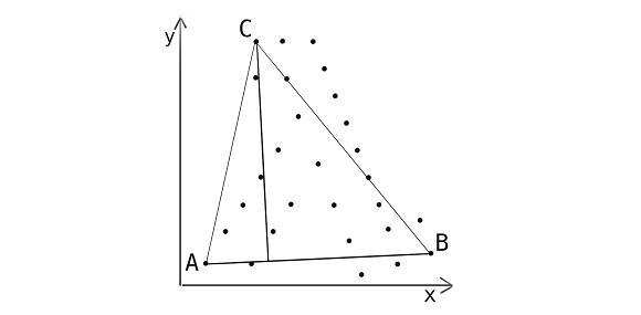
- First, we find the leftmost and rightmost points and draw a line between them dividing the space into two planes. We call the points A and B, respectively.
- Next, for each plane, we calculate distances between line AB and every point on the plane.
- We select the furthest point — let’s call it C — and make a triangle. By doing so we can ignore the points inside the triangle: they are clearly not going to form the convex hull.
- Repeat step 3 recursively for line AC and line BC until no points are left.
- Points A, B, C, and others that we found during step 4 are the ones that form the convex hull.
Before we continue further, I think I should make a short disclaimer. Quickhull is not the most efficient algorithm for computing the convex hull. Similarly to Quicksort it works as O(nLog(n)) on average and O(nˆ2) in a worst-case scenario. There are a couple of other algorithms that outperform Quickhull — for example, Graham’s Scan or Chan’s algorithm.
Our goal here is to make Quickhull run faster by parallelization. First, we will implement it naively, by the book, then parallelize it on the CPU, and finally, we modify and run it on the GPU.
Naive Implementation
To start with, we need to define a point model we are going to operate upon:
public readonly struct Point
{
  public float X { get; }
  public float Y { get; }

  public Point(float x, float y)
  {
    X = x;
    Y = y;
  }
}
Implementing Quickhull, we execute step 1 by finding the leftmost and rightmost points:
public HashSet<Point> QuickHull(Point[] points)
{
  if (points.Length <= 2) throw new ArgumentException($"Too little points: {points.Length}, expected 3 or more");

  var result = new HashSet<Point>();

  Point left = points[0], right = points[0];
  for (var i = 1; i < points.Length; i++)
  {
    if (points[i].X < left.X) left = points[i];
    if (points[i].X > right.X) right = points[i];
  }

  FindHull(points, left, right, 1, result);
  FindHull(points, left, right, -1, result);

  return result;
}
Following steps 2 and 3, we calculate distances between the line and all the points for each side of the line (1 and -1 above indicate the side). Finally, we find the maximum distance’s index, check it, and repeat the process recursively until we have no points left:
private static void FindHull(Point[] points, Point p1, Point p2, int side, HashSet<Point> result)
{
  var maxIndex = -1;
  var maxDistance = 0d;
  for (var i = 0; i < points.Length; i++)
  {
    if (Side(p1, p2, points[i]) != side) continue;

    var distance = Distance(p1, p2, points[i]);
    if (distance <= maxDistance) continue;

    maxIndex = i;
    maxDistance = distance;
  }

  if (maxIndex == -1)
  {
    result.Add(p1);
    result.Add(p2);
    return;
  }

  var newSide = Side(points[maxIndex], p1, p2);
  FindHull(points, points[maxIndex], p1, -newSide, result);
  FindHull(points, points[maxIndex], p2, newSide, result);
}
Here are the methods for calculating the distance and side:
private static double Distance(Point p1, Point p2, Point p)
{
  return Math.Abs((p.Y - p1.Y) * (p2.X - p1.X) - (p2.Y - p1.Y) * (p.X - p1.X));
}

private static int Side(Point p1, Point p2, Point p)
{
  var side = (p.Y - p1.Y) * (p2.X - p1.X) - (p2.Y - p1.Y) * (p.X - p1.X);
  if (side > 0) return 1;
  if (side < 0) return -1;
  return 0;
}
As you might have noticed, Distance method doesn’t return the actual distance between the point and the line. Instead, it returns a value that’s proportional to the distance. Since we only need to know which point is more distant, we can use this value further. For the lack of a better name, I’ll continue to call it “distance”.
CPU Parallelization
As you can see the algorithm iterates over the points array every time it divides a plane. It checks the side, computes distances between the points and the line, and finds the maximum distance’s index over and over again. Since we don’t have any data dependencies between iterations, we can parallelize these computations. We will do it by replacing the for loop with Parallel.For. So now FindHull looks like that:
private static void FindHull(Point[] points, Point p1, Point p2, int side, HashSet<Point> result)
{
  var maxIndex = -1;
  Parallel.For(0, points.Length, () => -1,
    (i, _, localMaxIndex) =>
    {
      if (Side(p1, p2, points[i]) != side) return localMaxIndex;

      var distance = localMaxIndex == -1 ? 0 : Distance(p1, p2, points[localMaxIndex]);
      if (Distance(p1, p2, points[i]) <= distance) return localMaxIndex;

      return i;
    },
    localMaxIndex =>
    {
      lock (Lock)
      {
        if (localMaxIndex == -1) return;
        var maxDistance = maxIndex != -1 ? Distance(p1, p2, points[maxIndex]) : 0;
        if (maxDistance < Distance(p1, p2, points[localMaxIndex]))
        {
          maxIndex = localMaxIndex;
        }
      }
    });

  if (maxIndex == -1)
  {
    result.Add(p1);
    result.Add(p2);
    return;
  }

  var newSide = Side(points[maxIndex], p1, p2);
  FindHull(points, points[maxIndex], p1, -newSide, result);
  FindHull(points, points[maxIndex], p2, newSide, result);
}
That’s a lot to take in, so let’s analyze each argument of Parallel.For:
- We still iterate over the points array starting from
0. - Naturally, we have to stop when we reach
points.Length. - Since we are looking for the furthest point’s index, we set its initial value to
-1, meaning not found. - The body of
Parallel.Forruns a lambda function in parallel that takes the current element, the internal state of the loop (we don’t really need it, hence_), and the current furthest point as arguments. The body of the lambda should look familiar. Essentially, it’s the same computation we did for the naive Quickhull. - Finally, the most interesting part. Each computed index is passed to a special function that applies it to the final result
maxIndex. It normally runs concurrently on multiple threads, therefore we have to play safe by using synchronization of some sort. Here we use our good old friendlock.
Since we do more work here by computing the same distance twice in steps 4 and 5, it might seem that the code should run slower. In fact, it runs faster, thanks to parallelization. To compare two implementations we will do a benchmark at the end of the post.
The rest of the implementation remains the same as in the naive version.
GPU Parallelization
Equipped with some knowledge on GPU computing and how to apply it in .NET, we can finally come closer to the title of the post — computing the convex hull on the GPU. Here we’re also going to parallelize the same loop as in the CPU version. It might not look as simple as the naive or CPU-parallelized versions, but I’ll try to keep things as simple as possible.
We start with the core idea of the implementation.
As stated at the beginning of the post, when running a kernel the GPU assigns it to the grid containing multiple blocks, each block being processed on a single SM. Instead of spawning as many threads as there are points, we are going to issue as many blocks as there are SMs on the GPU. Each block has a limited amount of threads, so in the grid we’ll only get numberOfBlocks * numberOfThreadsPerBlock threads at our disposal. Since this number might be smaller than the number of points, we’ll add an internal loop within each thread. Thus, each thread can do multiple iterations over the points array.
We’ll dedicate a thread to find its local maxIndex and maxDistance among the points it operates upon. Next, on the block level, we’ll figure out the block’s local maxIndex and maxDistance. Finally, we will pass this information to the host and compute the index of the furthest point there.
Let me illustrate how it works with a simple example. Say, we have a line [{ 0, 0 }, { 100, 100 }] and the following set of 7 points (for the sake of simplicity they are located on one side of the line):
A = { 15, 21 }
B = { 52, 94 }
C = { 52, 58 }
D = { 11, 90 }
E = { 45, 87 }
F = { 11, 98 }
G = { 33, 39 }
Suppose, we have a GPU that’s equipped with 2 SMs and has a block size of 2 threads. According to the idea, we issue 2 blocks having 4 threads in the grid overall (threads are denoted with a grid index):
Block0 = [Thread0, Thread1]
Block1 = [Thread2, Thread3]
Since we have more points than threads, we need to compute a stride that’s going to be applied to the thread’s internal loop. The stride is just the number of threads in the grid. So, Thread0 handles points A and D, Thread1 processes B and E, Thread2 takes C and F, and Thread3 works with G only. That leaves us with the following results on the thread level:
Thread0: maxIndex=4, maxDistance=4200
Thread1: maxIndex=5, maxDistance=8700
Thread2: maxIndex=2, maxDistance=600
Thread3: maxIndex=3, maxDistance=7900
Next, we find the block’s maxIndex and maxDistance. It would be:
Block0: maxIndex=5, maxDistance=8700
Block1: maxIndex=3, maxDistance=7900
In the end, we compare distances on the CPU and select the one with the highest value:
index=5, distance=8700That means that point F is the furthest in the set.
In order to implement the idea, we first need to refactor the body of QuickHull method by introducing some variables to help us with GPU operations:
public HashSet<Point> QuickHull(Point[] points)
{
  if (points.Length <= 2) throw new ArgumentException($"Too little points: {points.Length}, expected 3 or more");

  var result = new HashSet<Point>();

  var left = points[0];
  var right = points[0];
  for (var i = 1; i < points.Length; i++)
  {
    if (points[i].X < left.X) left = points[i];
    if (points[i].X > right.X) right = points[i];
  }

  using var context = new Context();
  context.EnableAlgorithms();

  using var accelerator = new CudaAccelerator(context);
  using var buffer = accelerator.Allocate<Point>(points.Length);
  buffer.CopyFrom(points, 0, 0, points.Length);

  FindHull(points, left, right, 1, result, accelerator, buffer.View);
  FindHull(points, left, right, -1, result, accelerator, buffer.View);

  return result;
}
The first part, in which we find the leftmost and rightmost points, should look familiar.
Next, we introduce the context and accelerator instances. ILGPU comes with battery included — it has an accompanying package ILGPU.Algorithms that contains a lot of useful GPU-enabled functions. We will use a couple of them later. Meanwhile, we need to tell ILGPU to use the library by calling EnableAlgorithms().
We allocate an additional buffer that’s used by the GPU to access points data. We only need it for reading, therefore we immediately copy data there and use it as a read-only view.
As in the previous implementations, we need to run FindHull for both sides of the line. This method has undergone some changes as well:
private static void FindHull(
  Point[] points,
  Point p1,
  Point p2,
  int side,
  HashSet<Point> result,
  Accelerator accelerator,
  ArrayView<Point> view)
{
  var (gridDim, groupDim) = accelerator.ComputeGridStrideLoopExtent(points.Length, out _);
  using var output = accelerator.Allocate<DataBlock<int, float>>(gridDim);

  var kernel = accelerator.LoadStreamKernel<
    ArrayView<Point>, int, Point, Point, ArrayView<DataBlock<int, float>>>
    (FindMaxIndexKernel);
  kernel(new KernelConfig(gridDim, groupDim), view, side, p1, p2, output);
  accelerator.Synchronize();

  var maxIndex = -1;
  var maxDistance = 0f;

  var candidates = output.GetAsArray();
  foreach (var candidate in candidates)
  {
    if (candidate.Item1 < 0) continue;
    FindMaxIndex(p1, p2, points[candidate.Item1], side, candidate.Item1, ref maxIndex, ref maxDistance);
  }

  if (maxIndex < 0)
  {
    result.Add(p1);
    result.Add(p2);
    return;
  }

  var newSide = Side(points[maxIndex], p1, p2);
  FindHull(points, points[maxIndex], p1, -newSide, result, accelerator, view);
  FindHull(points, points[maxIndex], p2, newSide, result, accelerator, view);
}
First, we ask the accelerator to compute gridDim (the number of blocks in the grid) and groupDim (the number of threads in blocks) based on the input size. (Since ILGPU insists on calling blocks “groups”, we will do that in code.) ComputeGridStrideLoopExtent also calculates the number of iterations per block and returns it as an out parameter, but we don’t really need it down the line.
Next, we allocate the output buffer where we store records of int and float computed within the blocks. The former refers to the index, and the latter — to the distance.
Then we load and run the kernel function providing the configuration. The kernel does computations in blocks and saves the result of each block into output. We will take a closer look at what’s going on there in a moment. Remember that we have to wait for the accelerator to do its job.
Once we get candidate points from output, it should be easy to compute the index of the furthest point and do the rest of the calculations. We did a similar job in previous implementations.
Now, perhaps, the most interesting part — the kernel body:
private static void FindMaxIndexKernel(
  ArrayView<Point> input,
  int side,
  Point a,
  Point b,
  ArrayView<DataBlock<int, float>> output)
{
  var stride = GridExtensions.GridStrideLoopStride;
  var maxIndex = -1;
  var maxDistance = 0f;

  for (var i = Grid.GlobalIndex.X; i < input.Length; i += stride)
  {
    FindMaxIndex(a, b, input[i], side, i, ref maxIndex, ref maxDistance);
  }

  var maxGroupDistance = GroupExtensions.Reduce<float, MaxFloat>(maxDistance);
  if (!maxDistance.Equals(maxGroupDistance))
  {
    maxIndex = -1;
  }

  var maxGroupIndex = GroupExtensions.Reduce<int, MaxInt32>(maxIndex);

  if (Group.IsFirstThread)
  {
    output[Grid.IdxX] = new DataBlock<int, float>(maxGroupIndex, maxGroupDistance);
  }
}
We obtain the stride of the thread loop by accessing the static property GridStrideLoopStride. As stated above, it should be equal to the number of blocks times their size. We also need to initialize thread’s maxIndex and maxDistance to -1 and 0f, respectively.
During the for loop, each thread accesses a point in the view applying the stride. It passes the point down to FindMaxIndex function which computes its index and distance and updates thread’s maxIndex and maxDistance.
Once we calculated indexes and distances on the thread level, we run the Reduce function from the algorithms library. It’s a block-wise operation that calls the execution barrier, takes provided values from all the threads within the block, and applies a reduction function to them. Once it’s done, it continues thread execution. Here we use it to find the maximum distance, that’s why we provide MaxFloat as a reduction function.
To find the index, though, we need to do a small trick. Within each thread, we reset maxIndex to -1 if thread’s maxDistance is not the maximum one on the block level. Then, to find the index we call Reduce, this time using MaxInt32 as a reduction function. As a result, we get either the initial -1, meaning we have no points left for this particular line or the index of the maximum distance.
Finally, we update output by adding a new record containing maxGroupIndex and maxGroupDistance. We can access a correct output index by using static Grid.IdxX property which returns a block index within the grid. Since we only need to update it once, we do it in the first thread.
FindMaxIndex that is used in both CPU and GPU code should look familiar as well:
private static void FindMaxIndex(
  Point a,
  Point b,
  Point candidatePoint,
  int side,
  int candidateIndex,
  ref int maxIndex,
  ref float maxDistance)
{
  if (Side(a, b, candidatePoint) != side) return;

  var candidateDistance = Distance(a, b, candidatePoint);
  if (candidateDistance <= maxDistance) return;

  maxIndex = candidateIndex;
  maxDistance = candidateDistance;
}
Benchmarking
Phew, it’s been a long ride! It is interesting to compare the implementations and see which one is faster.
For the benchmark, we will compute the convex hull of a set containing 10 million points. Not a very large input for a GPU, but it should be enough to see the performance difference.
Since hardware-specific code is involved, it’s also important to note the specs I use for benchmarking:
- BenchmarkDotNet=v0.12.1, OS=Windows 10 version 2004
- CPU=Intel Core i7-9750H CPU 2.60GHz (6 physical and 12 logic processors)
- GPU=GeForce GTX 1650 (16 multiprocessors and 896 CUDA cores)
- .NET Core SDK=3.1.402, .NET Core Runtime=3.1.8
|          Method |       Mean |    Error |   StdDev |
|---------------- |-----------:|---------:|---------:|
|           Naive | 2,779.5 ms | 28.85 ms | 25.58 ms |
| CpuParallelized | 1,155.2 ms | 22.94 ms | 43.09 ms |
| GpuParallelized |   210.2 ms |  3.72 ms |  5.22 ms |
Sweet! I wonder how would high-end graphics cards perform in this benchmark?
Conclusion
Usually, GPU programming finds its use in scientific computing, image processing, machine learning, and such. It’s probably not something that most of us, .NET developers, would use on a daily basis. However, it’s good to know that if there is a need for that, we can do it without leaving our comfortable .NET world. Whatever tools we choose for the job, though, we have to remember the main rule of performance tuning: always measure it. Especially when it comes to hardware-specific code.
Many thanks to MoFtZ for helping me a lot with index/distance GPU optimizations, to Alexei Matrosov for thoroughly reviewing this post, and to P J Łaszkowicz for suggesting numerous improvements.
You can check out the code from this post on GitHub: ComputingTheConvexHullOnGpu.